nf-core/circrna
circRNA quantification, differential expression analysis and miRNA target prediction of RNA-Seq data
Introduction
This document describes the output produced by the pipeline. Most of the plots are taken from the MultiQC report generated from the full-sized test dataset for the pipeline using a command similar to the one below:
nextflow run nf-core/circrna -profile test_full,<docker/singularity/institute>The directories listed below will be created in the results directory after the pipeline has finished. All paths are relative to the top-level results directory.
- references: Indices for various tools and intermediate reference genome files
- preprocessing: Per-sample concatenated FASTQ files
- quality_control
- fastqc: FastQC reports for raw reads
- trimgalore: Trim Galore! reports for trimmed reads
- bsj_detection
- combined: Combined BSJ calls across all samples
- samples: Per sample BSJ calls
- tools: Per tool and sample BSJ calls
- quantification
- combined: Quantification results for linear and circular transcripts across samples
- samples: Per sample quantification results
- transcriptome: Combined linear and circular transcriptome, based on GTF file and detected BSJs
- mirna_prediction
- binding_sites
- correlation
- mirna_expression
- statistical_tests
- circtest
- multiqc
- pipeline_info
Quality Control
FastQC
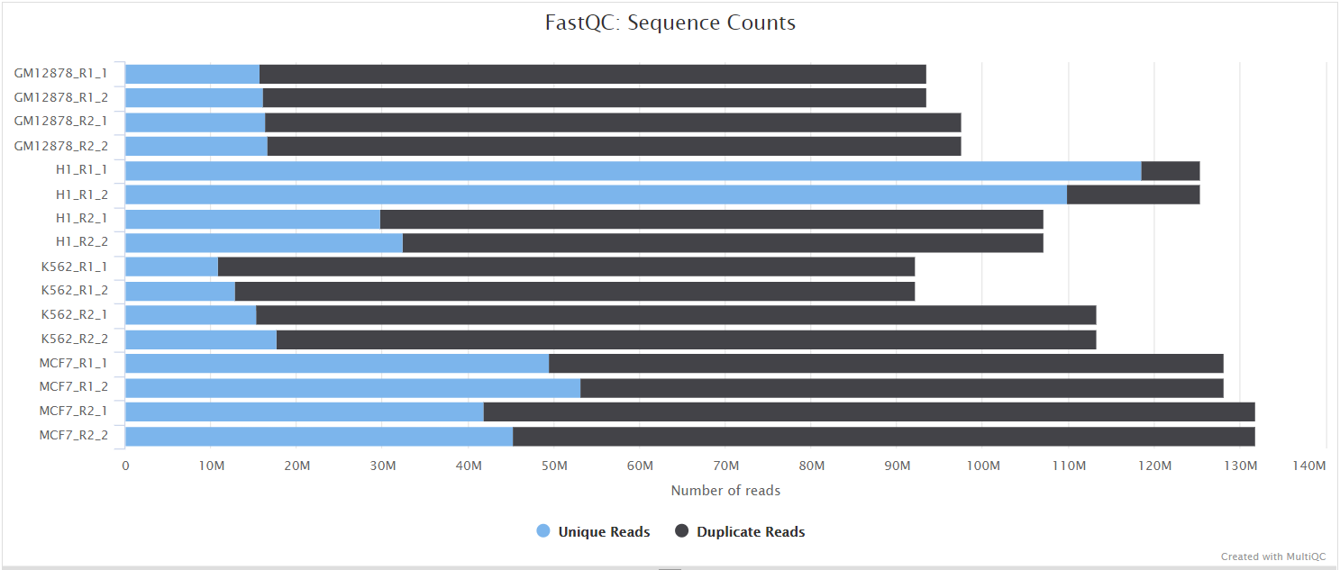
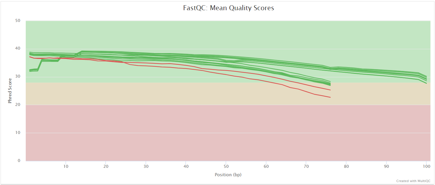
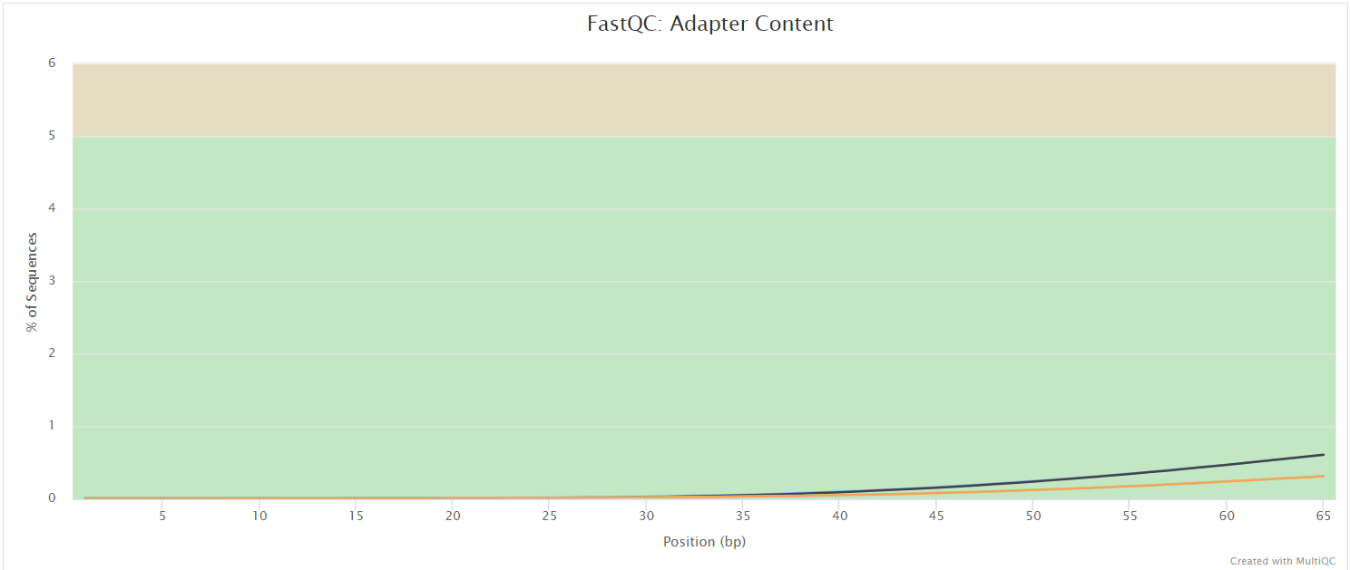
The FastQC plots displayed in the MultiQC report show untrimmed reads. They may contain adapter sequence and potentially regions with low quality.
Output files
fastqc/*_fastqc.html: FastQC report containing quality metrics.*_fastqc.zip: Zip archive containing the FastQC report, tab-delimited data file and plot images.
::: note The FastQC plots in this directory are generated relative to the raw, input reads. They may contain adapter sequence and regions of low quality. :::
FastQC gives general quality metrics about your sequenced reads. It provides information about the quality score distribution across your reads, per base sequence content (%A/T/G/C), adapter contamination and overrepresented sequences. For further reading and documentation see the FastQC help pages.
TrimGalore
Output files
trimgalore/*.fq.gz: If--save_trimmedis specified, FastQ files after adapter trimming will be placed in this directory.*_trimming_report.txt: Log file generated by Trim Galore!.
trimgalore/fastqc/*_fastqc.html: FastQC report containing quality metrics for read 1 (and read2 if paired-end) after adapter trimming.*_fastqc.zip: Zip archive containing the FastQC report, tab-delimited data file and plot images.
Trim Galore! is a wrapper tool around Cutadapt and FastQC to peform quality and adapter trimming on FastQ files. By default, Trim Galore! will automatically detect and trim the appropriate adapter sequence.

MultiQC
Output files
quality_control/MultiQC/Raw_Reads_MultiQC.html: Summary reports of unprocessed RNA-Seq reads.Trimmed_Reads_MultiQC.html: Summary reports of processed RNA-Seq reads.
MultiQC is a visualization tool that generates a single HTML report summarising all samples in your project. nf-core outputs HTML reports for sequencing read quality control.
Reference files
Output files
referencesindexbowtie: Directory containingBowtieindices.bowtie2: Directory containingBowtie2indices.bwa: Directory containingBWAindices.fasta: Directory containing FASTA index (.fai).hisat2: Directory containingHISAT2indices.segemehl: Directory containingSegemehlindex file.star: Directory containingSTARindices.
genomeclean_fasta: Directory containing a FASTA file with reduced headers, since MapSplice has problems with multiple header fields.filtered_gtf: Directory containing a GTF file with only entries that reside on chromosomes present in the reference FASTA file.chromosomes: Directory containing individual FASTA files for each chromosome.
bsh_detectioncircexplorer2: Directory containing theCIRCexplorer2annotation file.mapsplice: Directory containing theMapSpliceannotation file.
mirna_predictiontargetscan: Directory containing the TargetScan miRNA database.
nf-core/circrna will add the reference files to the output directory if save_reference is set to true. The resulting files, especially the aligner indices, can be used for speeding up future runs (if the resume option cannot be used). In order to achieve this, copy the indices to a location outside of the pipeline’s output directory and provide the path to the indices via the corresponding aligner flags (check the parameters documentation for more information).
Pipeline info
Output files
pipeline_info- Reports generated by Nextflow:
execution_report.html,execution_timeline.html,execution_trace.txtandpipeline_dag.dot/pipeline_dag.svg. - Reports generated by the pipeline:
pipeline_report.html,pipeline_report.txtandsoftware_versions.yml. Thepipeline_report*files will only be present if the--email/--email_on_failparameter’s are used when running the pipeline. - Parameters used by the pipeline run:
params.json.
- Reports generated by Nextflow:
BSJ detection
The rough workflow for the BSJ detection looks like this:
- Each tool detects BSJs in each sample and quantifies how many reads support each BSJ.
- Bring the tool outputs into a common format.
- Apply a threshold (parameter
bsj_reads) to the BSJ reads to filter out lowly supported BSJs. - Combine all tool-specific BSJ calls per sample into a single file.
- Filter out BSJs that are not supported by at least as many tools as specified by
min_tools. - Merge all samples into a single file. This now represents the “circular transcriptome”
Per tool
Output files available for all tools
unified: Directory containing the BSJ calls in the BED6 format.filtered: Based onunified, but filtered for BSJs with at leastbsj_readssupporting reads.masked: Based onfiltered, but scores are replaced by a dot (.)annotated: Based onmasked, but with additional columns for the circRNA type, the host gene(s), host transcript(s) and potential database hits. Contains a BED and a GTF file for each sample.fasta: Extracted sequences of the circRNAs in FASTA format. Based onmasked.intermediates: Contains intermediate files generated by the BSJ detection tools, as explained below.${tool}.csv: Number of reads that the tool found supporting the BSJ.
An exemption of the above is star, which is not used as a standalone BSJ detection tool, but the output of a 2-pass STAR alignment is used by CIRCexplorer2, circRNA finder and DCC.
CIRCexplorer2
Output files
bsj_detection/tools/circexplorer2/intermediates/${sample_id}/*.bed: Intermediate file generated byCIRCexplorer2 parsemodule, identifying STAR fusion junctions for downstream annotation.*.txt: Output files generated byCIRCexplorer2 annotatemodule, based on BED 12 format containing circRNA genomic location information, exon cassette composition and an additional 6 columns specifying circRNA annotations. Full descriptions of the 18 columns can be found in theCIRCexplorer2documentation.
CIRCexplorer2 uses *.Chimeric.out.junction files generated from STAR 2 pass mode to extract back-splice junction sites using the CIRCexplorer2 parse module. Following this, CIRCexplorer2 annotate performs re-alignment of reads to the back-splice junction sites to determine the precise positions of downstream donor and upstream acceptor splice sites. Back-splice junction sites are subsequently updated and annotated using the customised annotation text file.
circRNA finder
Output files
-
bsj_detection/tools/circrna_finder/intermediates/${sample_id}/*.filteredJunctions.bed: A bed file with all circular junctions found by the pipeline. The score column indicates the number reads spanning each junction.*.s_filteredJunctions.bed: A bed file with those junctions in*.filteredJunctions.bedthat are flanked by GT-AG splice sites. The score column indicates the number reads spanning each junction.*.s_filteredJunctions_fw.bed: A bed file with the same circular junctions as in file (b), but here the score column gives the average number of forward spliced reads at both splice sites around each circular junction.
circRNA finder uses *.Chimeric.out.sam, *.Chimeric.out.junction & *.SJ.out.tab from STAR 2nd pass files to identify circular RNAs in RNA-Seq data.
CIRIquant
Output files
bsj_detection/tools/ciriquant/intermediates/${sample_id}/*.log: ACIRIerror.logfile which should be empty, and a${sample_id}.logfile which contains the output log ofCIRIquant.*.bed:CIRI2output file in BED 6 format.*.gtf: Output file fromCIRIquantin GTF format. Full description of the columns available in theCIRIquantdocumentation.align/*.sorted.{bam, bam.bai}: (Sorted and indexed) bam file fromHISAT2alignment of RNA-Seq reads.
circ/*.ciri:CIRI2output file.*_denovo.sorted.{bam, bam.bai}: (Sorted and indexed) bam file fromBWAalignment of candidate circular reads to the pseudo reference.*_index.*.ht2:BWAindex files of the pseudo reference.*_index.fa: Reference FASTA file of candidate circular reads.
CIRIquant operates by aligning RNA-Seq reads using HISAT2 and CIRI2 to identify putative circRNAs. Next, a pseudo reference index is generated using bwa index by concatenating the two full-length sequences of the putative back-splice junction regions. Candidate circular reads are re-aligned against this pseudo reference using bwa mem, and back-splice junction reads are determined if they can be linearly and completely aligned to the putative back-splice junction regions.
DCC
Output files
/bsj_detection/tools/dcc/intermediates/${sample_id}/*.txt: Output file fromDCCcontaining position and BSJ read counts of circRNAs.
DCC identifies back-splice junction sites from *Chimeric.out.junction, *SJ.out.tab & *Aligned.sortedByCoord.out.bam files generated by STAR 2 pass mode, mapping the paired end reads both jointly and separately (STAR does not output read pairs that contain more than one chimeric junction thus a more granular approach is taken by DCC to fully characterise back-splice junctions in reads).
DCC then performs a series of filtering steps on candidate circular reads:
- Mapping of mates must be consistent with a circular RNA template i.e align to the back-splice junction.
- Filtering by a minimum number of junction reads per replicate (nf-core/circrna has set this parameter to
-Nr 1 1allowing all reads). - Circular reads are not allowed span more than one gene.
- Circular reads aligning to mitochondrial genome are removed.
- Circular reads that lack a canonical (GT/AG) splicing signal at the circRNA junction borders are removed.
Find circ
Output files
bsj_detection/tools/find_circ/intermediates/${sample_id}/*_anchors.qfa.gz: 20mer anchors extracted from unmapped reads.*_unmapped.bam: Unmapped RNA-Seq reads to reference genome.*.sites.bed: Output fromfind_circ, first six columns are in standard BED format. A description of the remaining columns is available in thefind_circdocumentation.*.sites.log: Summary statistics of candidate circular reads in the sample.*.sites.reads: Tab delimited file containing circRNA ID & sequence.
find circ utilises Bowtie2 short read mapper to align RNA-Seq reads to the genome. Reads that align fully and contiguously are discarded. Unmapped reads are converted to 20mers and aligned independently to find unique anchor positions within spliced exons - anchors that align in reverse orientation indicate circular RNA junctions. Anchor alignments are extended and must meet the following criteria:
- Breakpoints flanked by GT/AG splice sites.
- Unambiguous breakpoint detection.
- Maximum 2 mismatches in extension procedure.
- Breakpoint cannot reside more than 2nt inside a 20mer anchor.
- 2 reads must support the junction.
MapSplice
Output files
bsj_detection/tools/mapsplice/intermediates/${sample_id}/alignments.bam: Bam file containing aligned reads and fusion alignments.deletions.txt: Report of deletions.Fusion output files:fusions_raw.txt: raw fusion junctions without filteringfusion_candidates.txt: filtered fusion junctionsfusions_well_annotated.txt: annotated fusion junction candidates (align to annotation file provided)fusions_not_well_annotated.txt: fusions that do not align with supplied annotations
circular_RNAs.txt: circular RNAs reported.insertions.txt: Report of Insertions.junctions.txt: Reported splice junctions.stats.txt: Read alignment, Junction statistics.
MapSplice first splits reads into segments, and maps them to reference genome by using Bowtie. MapSplice attempts to fix unmapped segments as gapped alignments, with each gap corresponding to a splice junction. Finally a remapping step is used to identify back-spliced alignments that are in the presence of small exons.
Segemehl
Output files
bsj_detection/tools/segemehl/intermediates/${sample_id}/*.bam: Aligned reads in BAM format*.mult.bed: Thus, this bed file contains all splice events of a read. The start and end positions indicate the nucleotide after the first split (i.e. the beginning of the first intron) and the nucleotide before the last split (i.e. the end of the last intron), respectively. The name and score are equivalent to the one in the *.sngl file described above. The following fields 7 & 8 (thickStart and thickEnd) should be the identical to fields 2 & 3. Field 9 holds the color information for the item in RGB encoding (itemRGB). Field 10 (blockCount) indicates the number of splits represented by the BED item. Field 11 is a comma separated list of the intron sizes (blockSizes). Field 12 is the comma separated list of intron starts (blockStarts).*.sngl.bed: The bed file contains all single splice events predicted in the split read alignments.*.trns.bed: The custom text file contains all single split alignments predicted to be in trans, i.e. split alignments that are located on different chromosomes and/or different strands.
Segemehl implements split read alignment mode for reads that failed the attempt of collinear alignment. The algorithm will consider circular alignments. Circular splits are output to ${sample_id}.sngl.bed and parsed using customised scripts to produce counts representative of Segemehl quantification.
STAR
Output files
bsj_detection/tools/star1st_pass*.Aligned.out.bam: Coordinate sorted bam file containing aligned reads and chimeric reads.*.Chimeric.out.junction: Each line contains the details of chimerically aligned reads. Full descriptions of columns can be found inSTARdocumentation (section 5.4).*.Log.final.out: Summary mapping statistics after mapping job is complete, useful for quality control. The statistics are calculated for each read (single- or paired-end) and then summed or averaged over all reads.*.Log.out: Main log file with a lot of detailed information about the run. This file is most useful for troubleshooting and debugging.*.Log.progress.out: Reports job progress statistics, such as the number of processed reads, % of mapped reads etc.*.SJ.out.tab: High confidence collapsed splice junctions in tab-delimited form. Full description of columns can be found inSTARdocumentation (section 4.4).
2nd_pass*.Aligned.out.bam: Coordinate sorted bam file containing aligned reads and chimeric reads.*.Chimeric.out.junction: Each line contains the details of chimerically aligned reads. Full descriptions of columns can be found inSTARdocumentation (section 5.4).*.Chimeric.out.sam: Chimeric alignments in SAM format.*.Log.final.out: Summary mapping statistics after mapping job is complete, useful for quality control. The statistics are calculated for each read (single- or paired-end) and then summed or averaged over all reads.*.Log.out: Main log file with a lot of detailed information about the run. This file is most useful for troubleshooting and debugging.*.Log.progress.out: Reports job progress statistics, such as the number of processed reads, % of mapped reads etc.*.SJ.out.tab: High confidence collapsed splice junctions in tab-delimited form. Full description of columns can be found inSTARdocumentation (section 4.4).
sjdbdataset.SJ.out.tab: Chromosome, start, end & strand coordinates of novel splice junctions for all samples aligned using STAR 1st pass.
STAR in 2-pass mode is used to identify novel splice junctions in RNA-Seq data. The first pass of STAR is used to generate a genome index and align reads to the reference genome. The second pass of STAR uses the splice junctions identified in the first pass to align reads to the reference genome. This does not increase the number of detected novel junctions, but allows for more sensitive detection of splice reads mapping to novel junctions.
Per sample
Output files
bsj_detection/samples/${sample_id}/*.grouped.bed: Grouped BSJ calls in BED format. Score column represents the number of tools that support the BSJ.*.filtered.bed: Based on*.grouped.bed, but filtered for BSJs with at leastmin_toolssupporting tools.*.intersect_gtf.bed: Intersection of*.filtered.bedwith the reference GTF file. Intermediate file for annotation.*.intersect_database.bed: Intersection of*.filtered.bedwith the database BED file. Intermediate file for annotation.*.annotated.bed: Annotated BSJ calls in BED format, based on*.filtered.bed.*.annotated.gtf: Annotated BSJ calls in GTF format, based on*.filtered.bed.*.fa: Extracted sequences of the circRNAs in FASTA format, based on*.filtered.bed.*.upset.png: Sample-specific upset plot of BSJ calls across tools.
nf-core/circrna produces a sample-specific set of BSJ calls. The BSJ calls are filtered for BSJs with at least min_tools supporting tools. The filtered BSJ calls are then annotated with the reference GTF file and the database BED file. An upset plot is generated to visualise the overlap of BSJ calls across tools.
Combined
Output files
bsj_detection/combined/*.combined.bed: Unique BSJ calls across samples in BED format.*.intersect_gtf.bed: Intersection of*.filtered.bedwith the reference GTF file. Intermediate file for annotation.*.intersect_database.bed: Intersection of*.filtered.bedwith the database BED file. Intermediate file for annotation.*.annotated.bed: Annotated BSJ calls in BED format, based on*.filtered.bed.*.annotated.gtf: Annotated BSJ calls in GTF format, based on*.filtered.bed.*.fa: Extracted sequences of the circRNAs in FASTA format, based on*.filtered.bed.*.upset.png: Combined upset plot of BSJ calls across samples.
nf-core/circrna combines the sample-specific BSJ calls into a single file. The filtered BSJ calls are then annotated with the reference GTF file and the database BED file. An upset plot is generated to visualise the overlap of BSJ calls across tools.
Quantification
Since we now know the BSJ locations, we can now quantify their expression by mapping the reads to the region between the BSJ start and end coordinates. As each read can potentially originate from both linear and circular transcripts, the pipeline performs a joint quantification of the linear and circular transcriptome.
The quantification is performed using psirc-quant, which is a wrapper around kallisto. It allows for inferential-uncertainty aware quantification of linear and circular transcripts.
Transcriptome
Output files
quantification/transcriptome/*.combined.gtf: Combined linear and circular transcriptome in GTF format.*.filtered.gtf: Filtered linear and circular transcriptome in GTF format, based on*.combined.gtf.*.fasta: Combined linear and circular transcriptome in FASTA format, based on*.filtered.gtf.*.marked.fasta: Transcript sequences in FASTA format with the circRNA sequences marked with aCfield in the header.*.tx2gene.tsv: Transcript to gene mapping file.
Per sample
Output files
quantification/samples/${sample_id}/psirc*.abundance.h5: Abundance estimates in HDF5 format.*.abundance.tsv: Abundance estimates in TSV format.*.run_info.json: Run information in JSON format.pseudoalignments.bam: Pseudoalignments in BAM format.pseudoalignments.bai: Index file for pseudoalignments.
tximeta/*.rds: RDS file containing the the sample-specific transcript quantification data.
tximport/*.gene_counts_length_scaled.tsv: Gene counts scaled by transcript length.*.gene_counts_scaled.tsv: Gene counts scaled by library size.*.gene_counts.tsv: Gene counts.*.gene_lengths.tsv: Gene lengths.*.gene_tpm.tsv: Gene TPM values.*.transcript_counts.tsv: Transcript counts.*.transcript_lengths.tsv: Transcript lengths.*.transcript_tpm.tsv: Transcript TPM values.
nf-core/circrna performs quantification of linear and circular transcripts using psirc-quant. The quantification results are stored in HDF5 and TSV format. The pipeline also generates a tximeta RDS file containing the sample-specific transcript quantification data. The tximport directory contains gene and transcript counts, lengths and TPM values.
Combined
Output files
quantification/combined/gene_counts.csv: Count matrix of genes across samples.gene_tpm.csv: TPM matrix of genes across samples.tx_counts.csv: Count matrix of transcripts across samples.tx_tpm.csv: TPM matrix of transcripts across samples.linear.tsv: Count matrix of linear transcripts across samples.circular.tsv: Count matrix of circular transcripts across samples.experiments.merged.rds: RDS file containing a SummarizedExperiment with the merged transcript quantification data.
nf-core/circrna combines the sample-specific quantification results into proper count matrices. It also generates an RDS file containing a SummarizedExperiment with the merged transcript quantification data.
miRNA Prediction
Binding Sites
Tools
This section contains predicted binding sites for miRNA-target interactions generated by various computational tools. Each tool utilizes unique algorithms and criteria to identify potential miRNA binding sites on target genomic sequences, providing complementary insights into miRNA regulatory networks.
miRanda
Output files
mirna_prediction/bindingsites/tools/miranda/output*.miranda.txt: Raw predictions frommiRanda.
mirna_prediction/bindingsites/tools/miranda/unified*.miranda.tsv: Unified predictions frommiRanda.
miRanda performs miRNA target prediction of a genomic sequence against a miRNA database in 2 phases:
- First a dynamic programming local alignment is carried out between the query miRNA sequence and the reference sequence. This alignment procedure scores based on sequence complementarity and not on sequence identity.
- Secondly, the algorithm takes high-scoring alignments detected from phase 1 and estimates the thermodynamic stability of RNA duplexes based on these alignments. This second phase of the method utilises folding routines from the
RNAliblibrary, part of the ViennaRNA package.
TargetScan
Output files
mirna_prediction/bindingsites/tools/targetscan/output*.targetscan.txt: Raw predictions fromTargetScan.
mirna_prediction/bindingsites/tools/targetscan/unified*.targetscan.tsv: Unified predictions fromTargetScan.
TargetScan predicts biological targets of miRNAs by searching for the presence of conserved 8mer, 7mer, and 6mer sites within the circRNA mature sequence that match the seed region of each miRNA.
Targets
Output files
mirna_prediction/binding_sites/targets*_miRNA_targets.txt: Filtered target miRNAs of circRNAs called by quantification tools. Columns are self explanatory: miRNA, Score, Energy_KcalMol, Start, End, Site_type.
nf-core/circrna performs miRNA target filtering on miRanda and TargetScan predictions:
- miRNA must be called by both
miRandaandTargetScan. - If a site within the circRNA mature sequence shares duplicate miRNA ID’s overlapping the same coordinates, the miRNA with the highest score is kept.
Majority Vote
Output files
mirna_prediction/binding_sites/majority_votemirna.targets.tsv: Stores miRNA-target mappings with all targets listed per miRNA, making it compact and suitable for bulk analyses.mirna.majority.tsv: Lists each miRNA-target interaction on a separate line, which is helpful for detailed analysis of each interaction independently.
nf-core/circrna performs a majority vote on the predicted miRNA targets from TargetScan and miRanda based on a threshold specified by the user.
miRNA Expression
Output files
mirna_prediction/mirna_expression/mirna.normalized_counts.tsv: Contains normalized miRNA expression of all samples.mirna.normalized_counts_filtered.tsv: Contains miRNA expression after filtering.
nf-core/circrna processes miRNA expression data by normalizing and filtering it for further analysis.
Correlation
Output files
mirna_prediction/correlation*.tsv: Files named after the specific miRNA containing correlation results for that miRNA with its target transcripts.
nf-core/circrna computes correlations between miRNA and transcript expression levels and writes the results to individual TSV files for each miRNA-target interaction specified in the input binding sites file.